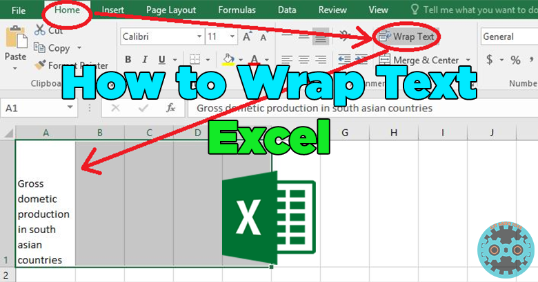
What is wrap text in Excel?
Wrap text in Excel is a technique that uses to break long lines of text into several lines. Every Excel user should know how to do it. In default long lines that we enter to the Excel, cell remain as one line. Wrapping instructs Excel to break long text into several lines inside the cells. In this scenario cell lengths not going to change but the height of the cell is changing. It increases automatically. If we change the cell width, the height and the text wrapping change spontaneously.
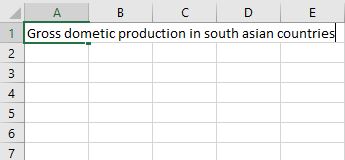
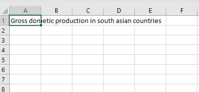
For example, cell A1 contains a long text value. But it covers cells B1, C1, D1, and E1. The text should be only in A1 text.
How to Wrap Text in Excel?
[g_article_ads]
There are few methods to do it. Let's see about them one by one.
Method 01: Wrapping a long text value using the Wrap Text button
- Select the cell or the range of cells.
- Then Go to the Home tab
- Click the Wrap Text button in the Alignment group
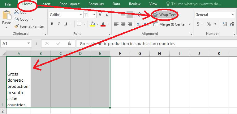
*You can change the column width by dragging the separator in between A and B. And also we can change the row height by dragging the separator in between row 1 and 2.
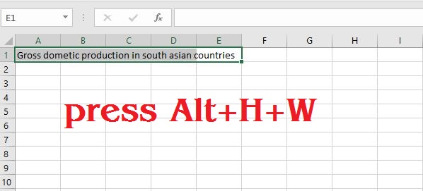
Method 02: Using short cut keys
- Select the cell or the range of cells.
- Then Press Alt+H+W
- This will apply the wrap in the text
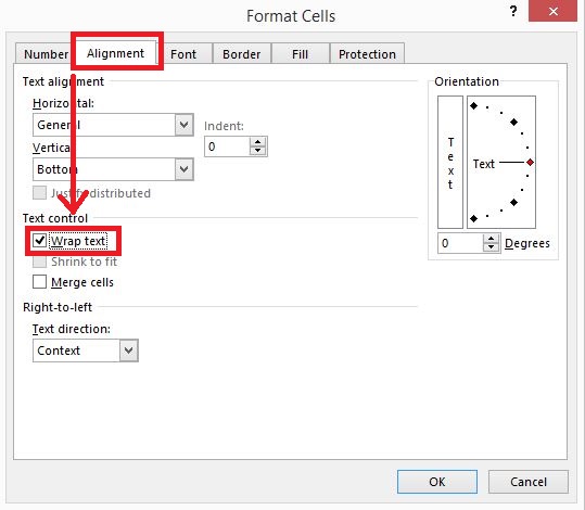
Method 03: Wrap using Format Cells dialog box
[g_article_ads]
- Select the cell or the range of cells
- Press Ctrl+1 to open the FORMAT CELLS dialog box
- Select the Alignment tab
- Select the Wrap Text checkbox in the text control section
- Then press Enter or click the OK button
Method 04: Manual Line break
Although we can wrap a text in a cell manually. To do that we should use the manual line break in Excel. Before we are going to that we should follow the below steps.
- select the cell and press F2 or double click in the cell to enter the formula bar.
- Place the cursor that where we want to break the line
- Press Alt+Enter
In this way, we can break the line number of times.

Author of Get Basic Idea – The knowledge base.
