How to change the background color of a cell base on the value in Excel

Excel is one of the important applications when analyzing data. Sometimes we have to need to add colors to cells base on the cell values to get a better analysis. In this tutorial, you can get a better understanding of how to add conditional formatting to specified cells and changing background colors of those base on formulas in an excel sheet. Follow the below steps.

Adding relevant colors to cells that are equal to the condition value.

Here is the Excel sheet which contains values related to colors.

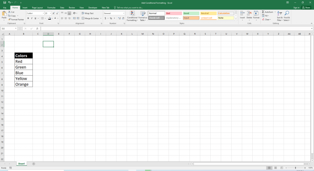
Step 1:

Select the range of cells to apply conditions.

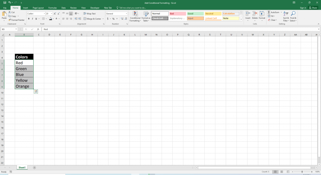
Step 2:

Go to Home tab >> Conditional Formatting >> Highlight Cell Rules >> Equal To, as per the below example.

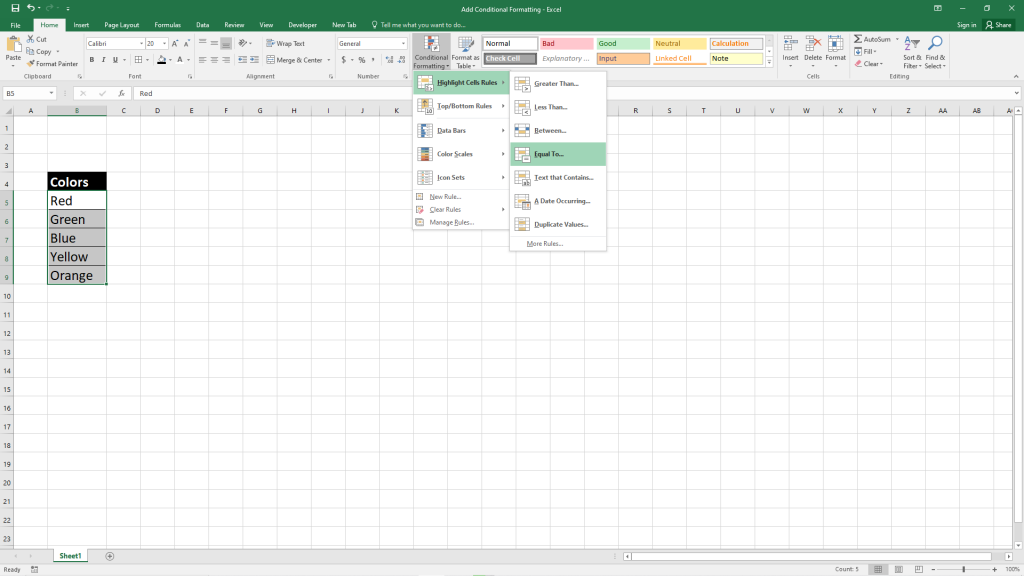
After you will see a coming popup window like below.

Step 3:

Give the value to format cells that are equal to the given value as per the below example.

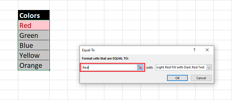
Step 4:

You can choose the default formatting options or custom format by drill down the right side field in popup windows as per the below example.

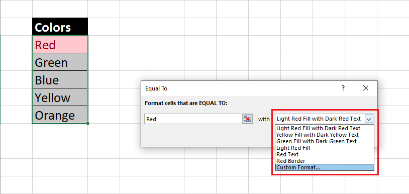
After choosing the custom format option, you will see custom format the setting window

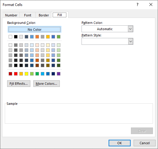
Step 5:

There are many formatting options in the custom format window. In the Fill tab, you can select the background colors as you want. After the selection click the OK button on all popped windows.

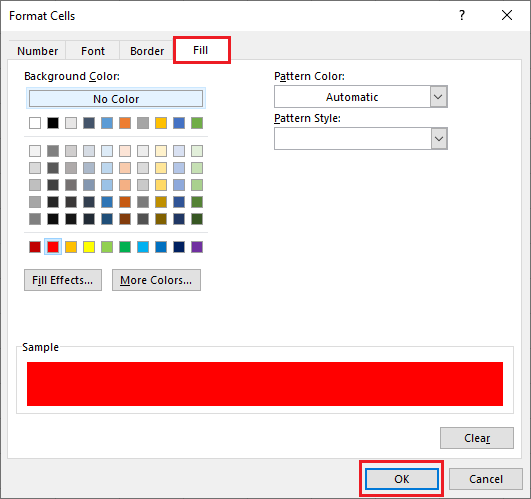
You can add the colors to each cell value by repeating these steps. For your knowledge, I have added the five colors matching with the cell values.

After adding colors to cells in the Excel sheet by the conditional formatting

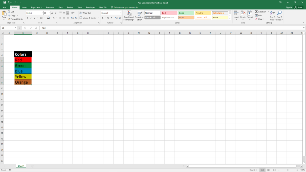
The background colors of the selected cell range will be changing dynamically when changing their values.

What are the other options available for adding conditional formatting?

There are multiple options have to add conditional formatting in Excel.

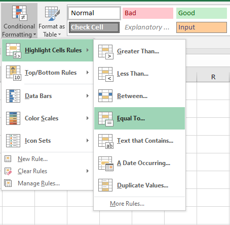
Let's see how to help these options to add conditions to format cells.

1. Greater Than

If the values of the selected cells are greater than a given value, the related format will be applied to those.

2. Less Than

If the values of the selected cells are less than a given value, the related format will be applied to those.

3. Between

If the values of the selected cells are between given values, the related format will be applied to those.

4. Equal To

If the values of the selected cells are equal to the given value, the related format will be applied to those. You got the idea about this option beginning.

5. Text that Contains

If the values of the selected cells contain the given value, the related format will be applied to those.

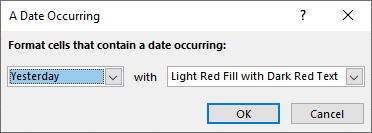
6. A Date Occurring

If the values of the selected cells contain occurring the given value, the related format will be applied to those. This applies only to the cells containing dates.

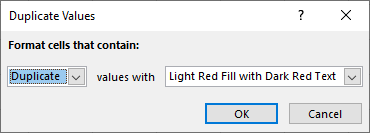
7. Duplicate Values

There are two options, Duplicate and Unique. If you select Duplicate, If the values of the selected cells are duplicates, the related format will be applied to those. If you select Unique, conditional formatting will be effected to unique values.

8. More Rules

In this option, you can give custom formulas to apply conditional formatting to selected cells.

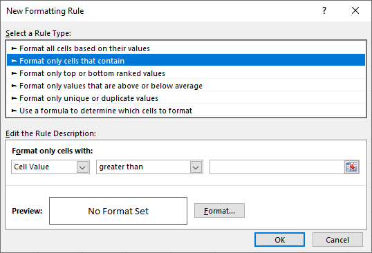
In the future, we will discuss how to use formulas to apply conditional formatting to cells in an Excel sheet. I hope you got a better understanding of conditional formatting and get in touch with futures posts to get more knowledge.